
ferra solutions
Lacuna

You can find this challenge here
but hurry, it ends in June July.
Note that I have no affiliation with this whatsoever.
In fact, I am also competing in this at present.
I prepared a nice CNN starter kit for this challenge which you can download below.
This gives you the whole kaboodle, from preprocessing data to creating a final submission file.
It is therefore quite elaborate but also easy to customise.
If you use this I would love to hear from you!
Perhaps best is to use the forums over at Zindi or else use the eMail provided on this page (under the big, blue logo).
Also included is the output that this will produce. Herewith the files.
- CNN starter workbook here
- Yawn. If your broswer opens this then right click on it and save-as it somewhere.
- Output it will produce here
Model overview below

This combines images from both RGB and Spectral photos and is called a siamese network.
Accuracy and improving one’s model
How accurate should one be and how can one improve one’s model. Herewith some ideas.
In this challenge the answer we need to provide is the plot centre - not in pixels but in ‘original’ coordinates.
We have images made up of pixels and thus the closest we can get to the centre is measured in pixels, and there is significant rounding at play.
Suppose you have a model that attaches a probability to each of the pixels in the image. This can be illustrated as shown in this image.
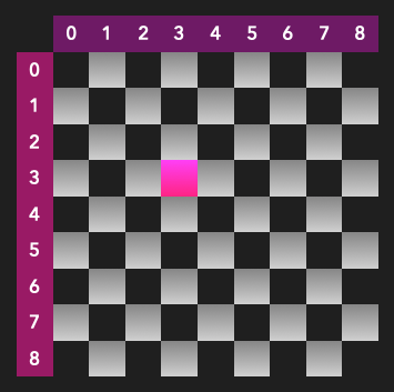
Suppose the model attaches a probability to each pixel of being the plot centre and it does so perfectly. Now, even with the perfect model, given the rounding at play, you will still have a MAE of 0.015! This can be calculated using the notebook given below - here is relevant the output from that notebook.
![]()
This 0.015 number is significant. The difference between the first and the 80th position on the leaderboard at the time of writing is around 0.015.
If, in stead of simply taking the pixel with highest probability, you convolve the pixels using a 2x2 square to find the centre accurate to 0.5 a pixel, you can improve this a lot.
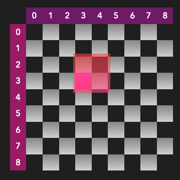
As shown in that notebook, this approach will improve the MAE of the perfect model significantly - to 0.008! At the time of writing, the difference between the best and 10th model is roughly 0.008.
If the model is indeed perfect, then it is easily possible to interpolate more accurately.
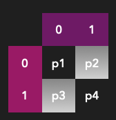
Earlier I used the perfect model simply to find the ‘perfect’ 2x2 square and used that to interpolate to the relevant half pixel. However, I could e.g. use the probabilities to interpolate even finer. In the image above, suppose
p1
is the highest. Rather than simply using pixels
( 0, 0 )
as solution I could look at the ratios between p1 and p2 and p3 and so on to interpolate to a higher degree of accuracy by reporting some fraction as answer.
The notebook used to perform these calculations can be found here .